Getting Answers while Data is Sparse Act 1: Promises and Baseball
Act 1: Promise
Any good story starts with several promises. That works for data stories too, as you’ll see. Let’s make those now.
- Promise of a world
- Promise of a character
- Promise of a voice
- Promise of a problem
- Promise of an event
Promise of a world
The whole world? No, just the world we want to understand. This is the world of bank transactions, of software development, customer conversion. This world has a purpose or goal. To understand how much the transactions will be before the authorization holds are cleared. To understand the rate of development or the security problems remaining. To understand relatable benfits and rates of conversion.
We’ll talk more about the elements of our world, outlining the sources, flows, and interconnections in the world. Our models give us insight into these parts of our world.
Promise of a character
Of all the purposes in our world, we choose one and deliver on that. Maybe it’s a stretch to use a framework for literature in our data work. However, I find that some of the more effective data models are very clear what a win looks like. That means they pick one very specific point of view and examine it first.
This gets a little easier if we consider the point of view needed by our boss, our team, our customer. Whoever is first going to examine our model.
Promise of a voice
We have a particular voice when we explain things. When the data is sparse, we have to be even more clear about how we are approaching the problem. The goal is to be insightful without getting carried away.
Now I should explain, by sparse data, I first mean a scarcity of rows of data. We can use these methods if we are dealing with missing values, but that’s a clever and advanced use of these tools, and we’re not going there today. Also, I’m not even convinced that this would always be a good idea.
Primarily, the voice needs to be clear. What particular view do we have about probability? A Bayesian one. What does that mean? It is the likelihood we believe so far. It is not the estimated truth that a more-careful scientist might publish.
I don’t think this approach to our work in any way demeans us. But it does introduce subjectivity into our work. What do we personally think is happening here? What could possibly have produced the data we have? Can we ask people more-knowledgeable than ourselves? Maybe an expert in the field, or a well-edited or peer-reviewed article? Can we find people that have something at stake that are willing to share their perspective?
We also need to combine the subjective sources of information with the empirical ones, the data. We combine these elements as probability distributions and parameters to those distributions. We combine our probability distributions into graphs to form joint distributions.
These tools produce something we call a generative model. In probability and statistics, a generative model is a model for randomly generating observable data values, typically given some hidden parameters. It specifies a joint probability distribution over observation and label sequences[1]. That means we’re not only describing our world, but explaining how likely our world might be. This can also help identify areas where we’d like to gather more or better data.
Promise of a problem
A problem in our world takes us back to the purpose of our world. I’d like to explain the financial situation for my customers, say, or what messages resonate well with these customers. The problem is almost always that we don’t have enough data. We might not trust our data. We might not be very confident how we got our data. We might imagine alternative models that could describe our data. Or worse, we might be unable to imagine anything beyond our first impressions.
In all circumstances, there are things we don’t observe directly. These are generally parameters, but could also be variables or sub systems.
Note, the problem should never be that we don’t know where we’re going. We take time looking at the world we want to model, and decide on a purpose we want to promote.
Promise of an event
Everything leads up to an event. This typically is a decision that someone needs to make. We advise our customers, we produce features in our products, we write new copy and see how it performs. Whatever the event, we put something on the line: our money, time, and/or reputation.
It is really important to prepare for that event and stand up straight and face it. That means we need to publish our insights, or risk something if we are wrong. I love how Nate Silver approaches his work [2] [3]. He emphasized our preparation for the big events, by putting our money, time, and reputation on the line.
Beyond Promises
Making sure we have a clear delivery to a good data model doesn’t ensure we approach the problem well. For that, we want a different list. Here is an outside-in approach that may prove useful:
How do we think about the data? What could explain the things we are seeing? We covered this with the world question, but let’s get more specific. We should at least imagine a world of cause and effect. At least have an idea of what might be driving things.
How do we research the problem? What can we learn from phone calls and reading expert opinion? It’s more than having the conversation, it’s about boiling it down to at least a good guess. You think it’s about 50? Is it ever more than 75? More than 80? No? Below 20? Now you’ve got an estimated mean and standard deviation for a normal distribution.
How do we combine our knowledge into a graphical model? Which variable types do we use? Here we take our cause-effect guesses, combine them with variables, and end up with a graph, a model that describes your problem. It’s not shameful to review variable types at this stage too. You might find some are easier to understand and use, even if they’re not very precise.
How do we deliver a solution? How does our approach change the data we need to prepare? Now we’re talking about delivering something. This is the real value of having a data story perspective to our work: data visualizations, priorities, clear questions answered. These are the good times when it all comes together.
That’s about as long winded as I dare go. Let’s set up some models with some examples. We’ll start off with a batting average example. That will give us a chance to explain some of the tools generally. Next, we’ll take on a bank transaction problem and see if we can understand the relationship between the hold authorizations and transactions. Finally, let’s see if we can take a stab at some electoral college problems and seek insight there.
Batting Averages
Let’s say we’re watching a baseball game. Here comes someone new, just called up from the minors. Great. What’s going to happen?
Well, let’s pause for a moment. What world are we talking about? A world of baseball. We have a purpose too. We want our team to win. Now, if you’re really into the world of baseball, and you’re not just posing like I am, you’re going to know this stuff really well. You’ve probably already read up on this batter and have a sense of what’s going on.
That’s OK. Who’s our character? Our batter of course. We’re rooting for the new guy.
And our voice? Well, as I’ve already admitted, I don’t know baseball. But I want to approach the problem in terms of batting averages. I want to admit up front that I’m starting from ignorance. Whatever I produce, I need to make sure I can walk someone from my ignorance to my conclusions in an especially transparent way. If I were an expert talking with avid fans, I could skip some steps and just add the parts they don’t already know.
The problem I’m facing is if I just assume this new rookie has no experience in the majors, then their first at bat would mean they’re either going to be a 1000 or 0. If they have a streat of 5 at bats, we could really convince ourselves that this batter is quite something or terrible and should be sent back to the minors.
And the event? I should bet my buddies, or brag up the batter after the game. Just have fun with what’s going on and be confident with what I’ve learned. Maybe even get into a good hearted argument about things from my newly elevated perspective.
So that’s a long wind up. It gets my juices flowing. I’m pretty sure I’m winding up for some good conversations, so I better get my act together. I probably know enough to know if I’m faking it or making it. I’ll come back to this description as I review deliverables to make sure I’m keeping my promises on this model. I’ve also reduced all the things I could possibly do into a much narrower spectrum. It takes the wrong kind of pressure off and puts the more-useful kind of pressure in my back pocket for when I need it. So let’s ask our 4 questions.
How do we think about the data? Where did this come from? Well, a batting average is the ratio of the number of safe hits over the number of times at bat.
How do we research this problem? We’d like to get an idea of what these batting averages could be. If we ask around, we’d find out there are 162 games in the regular season in the major leagues. We’d expect somewhere around 620 at bats for our batter across these 162 games. This is just stuff that other people said on the Internet. We’d also learn that 270 is a normal batting average, probably not below 200 and not 350. Not very precise, maybe, since I don’t know how credible these people are, but probably more right than wrong.
Let’s pick a variable for this batting average. If we want, we could use a normal distribution. 270 is our mean, and say 200 is 70 is two standard deviations. That adjusts our knowledge a little, since it would give us a range between 200 and 340 instead of 350. Still, it gives us a central tendancy, a nice bell curve to explain about where this batter fits the world of baseball.
Now, let’s just pause for a minute and look at what we’re thinking about. This batter is probably about like the other players in the major leagues. We’re saying the world that produced this batter, from little leagues through the minor leagues is kind of systematic. As the pitchers and field got better, so did the batting. After lots of thousands of players, we’ve arrived at a world that we suspect produces a rather predictable batting skill. In fact, I also found this little tidbit that seems to support where we’re going with this [4]
The league batting average in Major League Baseball for 2004 was just higher than .266, and the all-time league average is between .260 and .275.
As a first introduction to some concepts, I’m comfortable starting with just one variable and a couple of parameters. If we were thinking about a whole team, we might reason about whether we’re talking about a pitcher, who typically are terrible batters, often in the 100s [5]. But we’re not going to do that, let’s just make sure you’ve got a grip on a few tools before we handle harder questions. That said, let’s take a quick look at our model so far.
First we load some tools.
%matplotlib inline

import numpy as np
import scipy as sp
import pandas as pd
import matplotlib.pyplot as plt
import seaborn as sns

from scipy.stats import norm

sns.set_style('white')
sns.set_context('talk')

np.random.seed(123)
Next, we produce some artificial data, based on our thinking so far.
mu = .270 # Subjective (estimated) mean batting average
sigma = .035 # Subjective (estimated) standard deviation
data = sigma * np.random.randn(200) + mu # 200 random samples of our variable
Finally, we take a look at what we have so far.
ax = plt.subplot()
sns.distplot(data, kde=False, ax=ax)
_ = ax.set(title='Histogram of artificial batting averages, Normal', xlabel='x', ylabel='# observations');
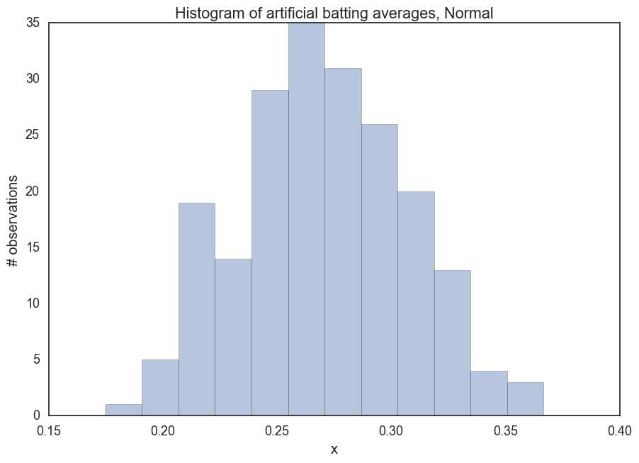
So, that looks about what we’d expect 200 baseball players’ batting averages to be. Maybe our standard deviation is a little high, but at least we’re getting from our minimal research and conclusions down to a measurable/sharable/understandable thing.
I Misled You
Sorry, not sorry.
We started with a normal distribution because the data we’ve seen looks kind of normal. There is a continuous range, they clump in the middle, and that’s all fine and nice. But what are we going to do once we see the batter bat? What new information do we have about the change in mean and standard deviation? If we had a season’s worth of data, we’d start to estimate these parameters and get a better sense of the kind of batter we’re talking about. But we’re wanting to have a bit of banter about our baseball insight, and somehow that’s probably not going to be good enough.
There’s another distribution that works a lot better on this sort of problem, the Beta distribution. In fact, this whole baseball conversation comes from a pretty interesting CrossValidated conversation that explains this distribution in beautiful detail [6].
A Beta distribution takes two parameters, alpha and beta. In our example, we set alpha to the number of times at bat when the batter gets on base, and beta to the rest of the times. (There’s got to be a more hip way to say that, I’ll keep working on my baseball voice.) Anyway, if we assume 300 times at bat, about a half a season, we get a fairly similar-looking outcome.
from scipy.stats import beta
a = 81 # Number of expected bases in a half season
b = 219 # Number of expected outs
r = beta.rvs(a, b, size=200) # 200 random variables from our distribution.
fig, ax = plt.subplots(1, 1)

x = np.linspace(beta.ppf(0.01, a, b),
              beta.ppf(0.99, a, b), 100)

sns.distplot(r, kde=False, ax=ax)
_ = ax.set(title='Histogram of artificial batting averages, Beta', xlabel='x', ylabel='# observations');
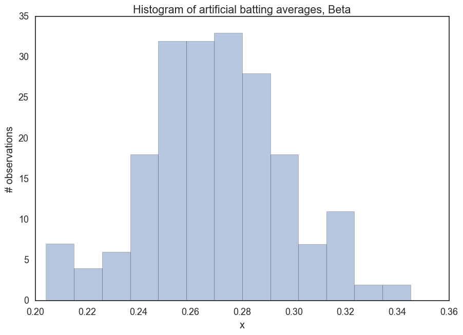
Notice how our upper and lower ranges look about right. Not below 200, not above 350. Notice how we centralize around the mean. What a useful distribution. We can take information we already have and convert it into a model for the information we’re looking for.
More importantly, this distribution works better with our sparse data problem. We’re saying we don’t know this player, so we’re assuming they’re about average. If we just record their at bat performance every time, we can easily update our beliefs about this batter’s ability. So, instead of alpha at 81 and beta at 219, we’d have an alpha at 82 if he gets on base or a beta at 220 if he doesn’t. We still believe he’s about average until we start to see some real evidence that we’re wrong. But this adjusts gradually. Small streaks don’t lead us to unreasonable conclusions.
Let’s look at a few examples of these.
a1 = 86 # A 5-hit streak
b1 = 219 # Number of outs
r1 = beta.rvs(a1, b1, size=200) # 200 random variables from our distribution.
fig, ax = plt.subplots(1, 1)

x = np.linspace(beta.ppf(0.01, a, b),
              beta.ppf(0.99, a, b), 100)

sns.distplot(r, kde=False, ax=ax)
sns.distplot(r1, kde=False, ax=ax)
_ = ax.set(title='Updated batting averages', xlabel='x', ylabel='# observations');

mean, var, skew, kurt = beta.stats(a, b, moments='mvsk')
mean1, var1, skew1, kurt1 = beta.stats(a1, b1, moments='mvsk')
df = pd.DataFrame(data={"Mean": [mean, mean1], "Variance": [var, var1], "Skew": [skew, skew1],
                       "Kurtosis": [kurt, kurt1]})
df
| Kurtosis | Mean | Skew | Variance | |
|---|---|---|---|---|
| 0 | 0.00138637347965 | 0.27 | 0.119047648134 | 0.000654817275748 |
| 1 | -0.00124390149534 | 0.281967213115 | 0.110441600404 | 0.000661639555043 |
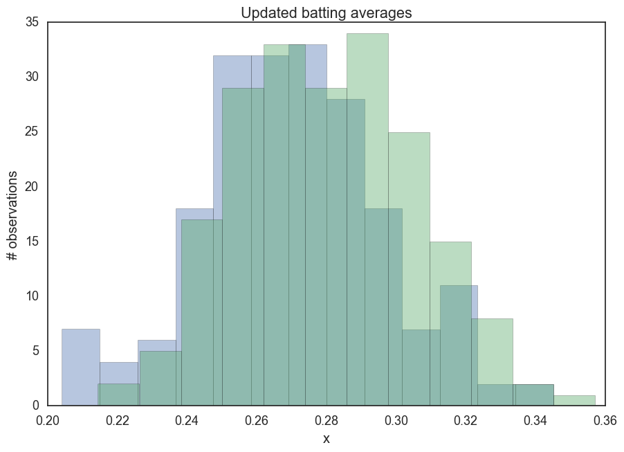
What we’re seeing is that even if the first at bats for a new rookie turn into a hitting streak, our belief in their batting ability is a 282, rather than a 1000. This seems about right for the kind of translation we had in mind between the world of baseball and this simple model.
So we’ve researched our problem with a little Google. We’ve represented our knowledge first in a normal distribution but made it easier to reason about it with a beta distribution. We actually have a graphical model with three nodes: our beta distribution and our alpha and beta parameters to that distribution.

The graphical model is a wonderful, but sometimes complicated thing. Our model happens to be directed, meaning we think that there are arrows from cause to effect. Parameters to a variable are very clearly direct causes to their distribution. We use a rather standard notation where parameters are dots and variables are circles.
We also added a distribution notation where ~B(alpha, beta) means a Beta distribution that takes an alpha and beta parameter. We could have also had a ~N(mu, sigma) for a normal distribution, ~P(lambda) for a Poisson distribution, etc. This is mostly there just to remind us what we’re doing when we come back to our model and need to remember what we’re up to.
So how do we present our knowledge? In this case, I’d say that the new rookie looks about as expected. If we’ve watched him for a few games, we’d comment on the difference between his performance and our expectations, but we’d be able to caution that we don’t know much yet. We’d likely be directed to look a little harder at his career leading up to the majors or listen more carefully to commentators that want to discuss his strengths and weaknesses from his past. We never hid the subjective nature of our conclusions, even though we have quantified what they are. We also walk away from this part of our work with some confidence that we’re able to reason about everything we see, and we’re not just being obstinate to win an argument. If we’re challenged seriously on our conclusions we could say that we’ll believe them when we see proof, but we’re pretty comfortable with our opinions so far.
We’re also keeping our promises. We’ve maintained our focus on a very simple view of a very limited world. We didn’t get pulled into all the other ways to discuss batting averages. We kept our focus on one character, just this new player. We’ve used a voice that starts to get us into baseball dicussions. We’ve been clear that our problem was figuring out batting averages with little or no data about a particular player. We anticipated the real event, which is the conversation we’re going to have with our friends who are baseball fans. This context makes our model a whole lot more satisfying, I think. We started with a fairly narrow interest and we were able to deliver on that interest. We could continue in this direction and probably do fairly well. In the context of a business problem or any data problem in any context, this kind of thinking should serve you well.
And now we’ve arrived at the end of Act 1, which is a good place for every Act 1 to end: at a crucial decision point. You’ll notice that there is a lot more to learn, a lot more to figure out. We need to get into much larger models, use more variable types, and deal with trickier problems. We’ll use PyMC and the excellent Probabilistic Programming and Bayesian Methods for Hackers. If you were to stop here, you could go back to your normal life and not upset things too much. But heroes take the challenge and experience a world view change through their adventures. So let’s go to Act 2 and see what’s waiting for us there.